Training PyTorch ResNet in your TensorFlow Projects

Framework Incompatibility

Practitioners with large codebases written in other frameworks, such as PyTorch, are unable to take advantage of TensorFlow’s rich ecosystem of state-of-the-art (SOTA) deployment toolings, as this requires converting their code manually and inaccurately.

Ivy’s transpiler allows ML practitioners to dynamically connect libraries, layers and models from different frameworks together. For PyTorch users, the transpiler provides a seamless and accurate way to introduce code written in PyTorch to TensorFlow pipelines.

In this blog post, we’ll go through an example of how the transpiler can be used to convert a model from PyTorch to TensorFlow and train the converted model in TensorFlow.

Transpiling a PyTorch model to TensorFlow

About the transpiled model

To illustrate a typical transpilation workflow, we’ll be converting a pre-trained ResNet model from PyTorch to TensorFlow, and using the transpiled model to run inference.

ResNet owes its name to its residual blocks with skip connections that enable the model to be extremely deep. Even though including skip connections is a common idea in the community now, it was a revolutionary architectural choice and allowed ResNet to reach up to 152 layers with no vanishing or exploding gradient problems during training.

Architecturally, a ResNet block is similar to a ConvNext block but differs in terms of the specific convolutional layers used, grouped convolution, normalization, activation function, and downsampling. Going through the details of the models is outside the scope of this demo, interested readers might want to go through the paper.

Installation

Since we want the packages to be available after installing, after running the first cell, the notebook will automatically restart.

You can then do Runtime -> Run all after the notebook has restarted, to run all of the cells.

Make sure you run this demo with GPU enabled!

!pip install -q ivy

!python3 -m pip install torchvision
!python3 -m pip install astor

exit()

Requirement already satisfied: torchvision in /usr/local/lib/python3.10/dist-packages (0.18.0+cu121)
Requirement already satisfied: numpy in /usr/local/lib/python3.10/dist-packages (from torchvision) (1.25.2)
Requirement already satisfied: torch==2.3.0 in /usr/local/lib/python3.10/dist-packages (from torchvision) (2.3.0+cu121)
Requirement already satisfied: pillow!=8.3.*,>=5.3.0 in /usr/local/lib/python3.10/dist-packages (from torchvision) (9.4.0)
Requirement already satisfied: filelock in /usr/local/lib/python3.10/dist-packages (from torch==2.3.0->torchvision) (3.15.3)
Requirement already satisfied: typing-extensions>=4.8.0 in /usr/local/lib/python3.10/dist-packages (from torch==2.3.0->torchvision) (4.12.2)
Requirement already satisfied: sympy in /usr/local/lib/python3.10/dist-packages (from torch==2.3.0->torchvision) (1.12.1)
Requirement already satisfied: networkx in /usr/local/lib/python3.10/dist-packages (from torch==2.3.0->torchvision) (3.3)
Requirement already satisfied: jinja2 in /usr/local/lib/python3.10/dist-packages (from torch==2.3.0->torchvision) (3.1.4)
Requirement already satisfied: fsspec in /usr/local/lib/python3.10/dist-packages (from torch==2.3.0->torchvision) (2023.6.0)
Requirement already satisfied: nvidia-cuda-nvrtc-cu12==12.1.105 in /usr/local/lib/python3.10/dist-packages (from torch==2.3.0->torchvision) (12.1.105)
Requirement already satisfied: nvidia-cuda-runtime-cu12==12.1.105 in /usr/local/lib/python3.10/dist-packages (from torch==2.3.0->torchvision) (12.1.105)
Requirement already satisfied: nvidia-cuda-cupti-cu12==12.1.105 in /usr/local/lib/python3.10/dist-packages (from torch==2.3.0->torchvision) (12.1.105)
Requirement already satisfied: nvidia-cudnn-cu12==8.9.2.26 in /usr/local/lib/python3.10/dist-packages (from torch==2.3.0->torchvision) (8.9.2.26)
Requirement already satisfied: nvidia-cublas-cu12==12.1.3.1 in /usr/local/lib/python3.10/dist-packages (from torch==2.3.0->torchvision) (12.1.3.1)
Requirement already satisfied: nvidia-cufft-cu12==11.0.2.54 in /usr/local/lib/python3.10/dist-packages (from torch==2.3.0->torchvision) (11.0.2.54)
Requirement already satisfied: nvidia-curand-cu12==10.3.2.106 in /usr/local/lib/python3.10/dist-packages (from torch==2.3.0->torchvision) (10.3.2.106)
Requirement already satisfied: nvidia-cusolver-cu12==11.4.5.107 in /usr/local/lib/python3.10/dist-packages (from torch==2.3.0->torchvision) (11.4.5.107)
Requirement already satisfied: nvidia-cusparse-cu12==12.1.0.106 in /usr/local/lib/python3.10/dist-packages (from torch==2.3.0->torchvision) (12.1.0.106)
Requirement already satisfied: nvidia-nccl-cu12==2.20.5 in /usr/local/lib/python3.10/dist-packages (from torch==2.3.0->torchvision) (2.20.5)
Requirement already satisfied: nvidia-nvtx-cu12==12.1.105 in /usr/local/lib/python3.10/dist-packages (from torch==2.3.0->torchvision) (12.1.105)
Requirement already satisfied: triton==2.3.0 in /usr/local/lib/python3.10/dist-packages (from torch==2.3.0->torchvision) (2.3.0)
Requirement already satisfied: nvidia-nvjitlink-cu12 in /usr/local/lib/python3.10/dist-packages (from nvidia-cusolver-cu12==11.4.5.107->torch==2.3.0->torchvision) (12.5.40)
Requirement already satisfied: MarkupSafe>=2.0 in /usr/local/lib/python3.10/dist-packages (from jinja2->torch==2.3.0->torchvision) (2.1.5)
Requirement already satisfied: mpmath<1.4.0,>=1.1.0 in /usr/local/lib/python3.10/dist-packages (from sympy->torch==2.3.0->torchvision) (1.3.0)
Collecting astor
  Downloading astor-0.8.1-py2.py3-none-any.whl (27 kB)
Installing collected packages: astor
Successfully installed astor-0.8.1

Setting-up the source model

We import the necessary libraries. We’ll mostly use the PyTorch’s Torchvision API to load the model, Ivy to transpile it from PyTorch to TensorFlow, and TensorFlow functions to fine-tune the transpiled model.

import warnings
warnings.filterwarnings("ignore")
import logging
import tensorflow as tf
try:
   tf.config.experimental.set_memory_growth(
      tf.config.list_physical_devices("GPU")[0], True
   )
except:
   pass

# Filter TensorFlow info and warning messages
tf.get_logger().setLevel(logging.ERROR)
import os
import ivy
ivy.set_default_device("gpu:0")
import torch
import torchvision
from torchvision import datasets, models, transforms

torch.manual_seed(0)
tf.random.set_seed(0)

2024-10-21 17:50:39.195130: I tensorflow/core/util/port.cc:153] oneDNN custom operations are on. You may see slightly different numerical results due to floating-point round-off errors from different computation orders. To turn them off, set the environment variable `TF_ENABLE_ONEDNN_OPTS=0`.
2024-10-21 17:50:39.374700: E external/local_xla/xla/stream_executor/cuda/cuda_fft.cc:485] Unable to register cuFFT factory: Attempting to register factory for plugin cuFFT when one has already been registered
2024-10-21 17:50:39.441741: E external/local_xla/xla/stream_executor/cuda/cuda_dnn.cc:8454] Unable to register cuDNN factory: Attempting to register factory for plugin cuDNN when one has already been registered
2024-10-21 17:50:39.461396: E external/local_xla/xla/stream_executor/cuda/cuda_blas.cc:1452] Unable to register cuBLAS factory: Attempting to register factory for plugin cuBLAS when one has already been registered
2024-10-21 17:50:39.592512: I tensorflow/core/platform/cpu_feature_guard.cc:210] This TensorFlow binary is optimized to use available CPU instructions in performance-critical operations.
To enable the following instructions: AVX2 AVX_VNNI FMA, in other operations, rebuild TensorFlow with the appropriate compiler flags.
2024-10-21 17:50:40.820737: W tensorflow/compiler/tf2tensorrt/utils/py_utils.cc:38] TF-TRT Warning: Could not find TensorRT
WARNING: All log messages before absl::InitializeLog() is called are written to STDERR
I0000 00:00:1729515043.033296    4399 cuda_executor.cc:1001] could not open file to read NUMA node: /sys/bus/pci/devices/0000:01:00.0/numa_node
Your kernel may have been built without NUMA support.
2024-10-21 17:50:43.058149: W tensorflow/core/common_runtime/gpu/gpu_device.cc:2343] Cannot dlopen some GPU libraries. Please make sure the missing libraries mentioned above are installed properly if you would like to use GPU. Follow the guide at https://www.tensorflow.org/install/gpu for how to download and setup the required libraries for your platform.
Skipping registering GPU devices...
WARNING:root:   Some binaries seem to be missing in your system. This could be either because we don't have compatible binaries for your system or that newer binaries were available. In the latter case, calling ivy.utils.cleanup_and_fetch_binaries() should fetch the binaries binaries. Feel free to create an issue on https://github.com/ivy-llc/ivy.git in case of the former

WARNING:root:
Following are the supported configurations :
compiler : cp38-cp38-manylinux_2_17_x86_64, cp38-cp38-win_amd64, cp39-cp39-manylinux_2_17_x86_64, cp39-cp39-win_amd64, cp310-cp310-manylinux_2_17_x86_64, cp310-cp310-win_amd64, cp310-cp310-macosx_12_0_arm64, cp311-cp311-manylinux_2_17_x86_64, cp311-cp311-win_amd64, cp311-cp311-macosx_12_0_arm64, cp312-cp312-manylinux_2_17_x86_64, cp312-cp312-win_amd64, cp312-cp312-macosx_12_0_arm64

Load the Data

We will use torchvision and torch.utils.data packages for loading the data.

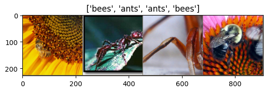
The problem we’re going to solve today is to train a model to classify ants and bees. We have about 120 training images each for ants and bees. There are 75 validation images for each class. Usually, this is a very small dataset to generalize upon, if trained from scratch. Since we are using transfer learning, we should be able to generalize reasonably well.

This dataset is a very small subset of imagenet.

Note: Download the data from here and extract it to the current directory by running the following cell

import requests
import os
import zipfile

# URL of the zip file you want to download
url = 'https://download.pytorch.org/tutorial/hymenoptera_data.zip'  # Replace with your URL

# Send a GET request to the URL
response = requests.get(url)

# Check if the request was successful (status code 200)
if response.status_code == 200:
    # Get the file name from the URL
    filename = os.path.basename(url)

    # Specify where you want to save the zip file (current working directory in Colab)
    zip_save_path = os.path.join(os.getcwd(), filename)

    # Write the content to the zip file
    with open(zip_save_path, 'wb') as f:
        f.write(response.content)

    print(f"Zip file downloaded successfully as '{filename}' in the current working directory.")

    # Extract the contents of the zip file
    with zipfile.ZipFile(zip_save_path, 'r') as zip_ref:
        zip_ref.extractall(os.getcwd())

    print("Zip file contents extracted successfully.")

    # Optionally, you can remove the zip file after extraction
    os.remove(zip_save_path)
    print(f"Zip file '{filename}' deleted.")

else:
    print(f"Failed to download zip file from '{url}'. Status code: {response.status_code}")

Zip file downloaded successfully as 'hymenoptera_data.zip' in the current working directory.
Zip file contents extracted successfully.
Zip file 'hymenoptera_data.zip' deleted.

# Data augmentation and normalization for training
# Just normalization for validation
data_transforms = {
    'train': transforms.Compose([
        transforms.RandomResizedCrop(224),
        transforms.RandomHorizontalFlip(),
        transforms.ToTensor(),
        transforms.Normalize([0.485, 0.456, 0.406], [0.229, 0.224, 0.225])
    ]),
    'val': transforms.Compose([
        transforms.Resize(256),
        transforms.CenterCrop(224),
        transforms.ToTensor(),
        transforms.Normalize([0.485, 0.456, 0.406], [0.229, 0.224, 0.225])
    ]),
}

data_dir = 'hymenoptera_data'

image_datasets = {
    x: datasets.ImageFolder(
        os.path.join(data_dir, x), data_transforms[x]
    ) for x in ['train', 'val']
}

dataloaders = {
    x: torch.utils.data.DataLoader(
        image_datasets[x], batch_size=4,
        shuffle=True,
        num_workers=4
    ) for x in ['train', 'val']
}

dataset_sizes = {x: len(image_datasets[x]) for x in ['train', 'val']}
class_names = image_datasets['train'].classes
device = torch.device("cuda:0" if torch.cuda.is_available() else "cpu")

Visualize a few images

We also load an input tensor to be passed as the input for transpilation

import numpy as np
from matplotlib import pyplot as plt


def imshow(inp, title=None):
    """Display image for Tensor."""
    inp = inp.numpy().transpose((1, 2, 0))
    mean = np.array([0.485, 0.456, 0.406])
    std = np.array([0.229, 0.224, 0.225])
    inp = std * inp + mean
    inp = np.clip(inp, 0, 1)
    plt.imshow(inp)
    if title is not None:
        plt.title(title)
    plt.pause(0.001)  # pause a bit so that plots are updated


# Get a batch of training data
inputs, classes = next(iter(dataloaders['train']))

# Make a grid from batch
out = torchvision.utils.make_grid(inputs)

imshow(out, title=[class_names[x] for x in classes])

Load the pre-trained model

We then initialise our ML model through the torchvision API, specifically we’ll be using ResNet18. Note that while we are using a model from the torchvision models API for this demonstration, it would still work with any arbitrary PyTorch model regardless of how it is being loaded. You can load models hosted on different platforms including local models.

model = torchvision.models.resnet18(weights='IMAGENET1K_V1')
model

ResNet(
  (conv1): Conv2d(3, 64, kernel_size=(7, 7), stride=(2, 2), padding=(3, 3), bias=False)
  (bn1): BatchNorm2d(64, eps=1e-05, momentum=0.1, affine=True, track_running_stats=True)
  (relu): ReLU(inplace=True)
  (maxpool): MaxPool2d(kernel_size=3, stride=2, padding=1, dilation=1, ceil_mode=False)
  (layer1): Sequential(
    (0): BasicBlock(
      (conv1): Conv2d(64, 64, kernel_size=(3, 3), stride=(1, 1), padding=(1, 1), bias=False)
      (bn1): BatchNorm2d(64, eps=1e-05, momentum=0.1, affine=True, track_running_stats=True)
      (relu): ReLU(inplace=True)
      (conv2): Conv2d(64, 64, kernel_size=(3, 3), stride=(1, 1), padding=(1, 1), bias=False)
      (bn2): BatchNorm2d(64, eps=1e-05, momentum=0.1, affine=True, track_running_stats=True)
    )
    (1): BasicBlock(
      (conv1): Conv2d(64, 64, kernel_size=(3, 3), stride=(1, 1), padding=(1, 1), bias=False)
      (bn1): BatchNorm2d(64, eps=1e-05, momentum=0.1, affine=True, track_running_stats=True)
      (relu): ReLU(inplace=True)
      (conv2): Conv2d(64, 64, kernel_size=(3, 3), stride=(1, 1), padding=(1, 1), bias=False)
      (bn2): BatchNorm2d(64, eps=1e-05, momentum=0.1, affine=True, track_running_stats=True)
    )
  )
  (layer2): Sequential(
    (0): BasicBlock(
      (conv1): Conv2d(64, 128, kernel_size=(3, 3), stride=(2, 2), padding=(1, 1), bias=False)
      (bn1): BatchNorm2d(128, eps=1e-05, momentum=0.1, affine=True, track_running_stats=True)
      (relu): ReLU(inplace=True)
      (conv2): Conv2d(128, 128, kernel_size=(3, 3), stride=(1, 1), padding=(1, 1), bias=False)
      (bn2): BatchNorm2d(128, eps=1e-05, momentum=0.1, affine=True, track_running_stats=True)
      (downsample): Sequential(
        (0): Conv2d(64, 128, kernel_size=(1, 1), stride=(2, 2), bias=False)
        (1): BatchNorm2d(128, eps=1e-05, momentum=0.1, affine=True, track_running_stats=True)
      )
    )
    (1): BasicBlock(
      (conv1): Conv2d(128, 128, kernel_size=(3, 3), stride=(1, 1), padding=(1, 1), bias=False)
      (bn1): BatchNorm2d(128, eps=1e-05, momentum=0.1, affine=True, track_running_stats=True)
      (relu): ReLU(inplace=True)
      (conv2): Conv2d(128, 128, kernel_size=(3, 3), stride=(1, 1), padding=(1, 1), bias=False)
      (bn2): BatchNorm2d(128, eps=1e-05, momentum=0.1, affine=True, track_running_stats=True)
    )
  )
  (layer3): Sequential(
    (0): BasicBlock(
      (conv1): Conv2d(128, 256, kernel_size=(3, 3), stride=(2, 2), padding=(1, 1), bias=False)
      (bn1): BatchNorm2d(256, eps=1e-05, momentum=0.1, affine=True, track_running_stats=True)
      (relu): ReLU(inplace=True)
      (conv2): Conv2d(256, 256, kernel_size=(3, 3), stride=(1, 1), padding=(1, 1), bias=False)
      (bn2): BatchNorm2d(256, eps=1e-05, momentum=0.1, affine=True, track_running_stats=True)
      (downsample): Sequential(
        (0): Conv2d(128, 256, kernel_size=(1, 1), stride=(2, 2), bias=False)
        (1): BatchNorm2d(256, eps=1e-05, momentum=0.1, affine=True, track_running_stats=True)
      )
    )
    (1): BasicBlock(
      (conv1): Conv2d(256, 256, kernel_size=(3, 3), stride=(1, 1), padding=(1, 1), bias=False)
      (bn1): BatchNorm2d(256, eps=1e-05, momentum=0.1, affine=True, track_running_stats=True)
      (relu): ReLU(inplace=True)
      (conv2): Conv2d(256, 256, kernel_size=(3, 3), stride=(1, 1), padding=(1, 1), bias=False)
      (bn2): BatchNorm2d(256, eps=1e-05, momentum=0.1, affine=True, track_running_stats=True)
    )
  )
  (layer4): Sequential(
    (0): BasicBlock(
      (conv1): Conv2d(256, 512, kernel_size=(3, 3), stride=(2, 2), padding=(1, 1), bias=False)
      (bn1): BatchNorm2d(512, eps=1e-05, momentum=0.1, affine=True, track_running_stats=True)
      (relu): ReLU(inplace=True)
      (conv2): Conv2d(512, 512, kernel_size=(3, 3), stride=(1, 1), padding=(1, 1), bias=False)
      (bn2): BatchNorm2d(512, eps=1e-05, momentum=0.1, affine=True, track_running_stats=True)
      (downsample): Sequential(
        (0): Conv2d(256, 512, kernel_size=(1, 1), stride=(2, 2), bias=False)
        (1): BatchNorm2d(512, eps=1e-05, momentum=0.1, affine=True, track_running_stats=True)
      )
    )
    (1): BasicBlock(
      (conv1): Conv2d(512, 512, kernel_size=(3, 3), stride=(1, 1), padding=(1, 1), bias=False)
      (bn1): BatchNorm2d(512, eps=1e-05, momentum=0.1, affine=True, track_running_stats=True)
      (relu): ReLU(inplace=True)
      (conv2): Conv2d(512, 512, kernel_size=(3, 3), stride=(1, 1), padding=(1, 1), bias=False)
      (bn2): BatchNorm2d(512, eps=1e-05, momentum=0.1, affine=True, track_running_stats=True)
    )
  )
  (avgpool): AdaptiveAvgPool2d(output_size=(1, 1))
  (fc): Linear(in_features=512, out_features=1000, bias=True)
)

Converting the model from PyTorch to TensorFlow

As we explain in our Quickstart Guide, transpiling a model (an instance of a trainable class) involves manually providing the type/class of the model rather than the model itself. This is because Ivy’s transpiler will eagerly convert all source code of the model from PyTorch to TensorFlow and make it readily available for you in the output directory (controlled by passing the output_dir kwarg to ivy.transpile, defaulting to ivy_transpiled_outputs/).

The weights of the transpiled model and the original model (if it was pretrained or loaded from a checkpoint) can be easily synced by using ivy.sync_models as we demonstrate in this demo

type(model)

torchvision.models.resnet.ResNet

TensorflowResNet = ivy.transpile(type(model), source="torch", target="tensorflow")

Initializing and building the TensorFlow model

from ivy_transpiled_outputs.tensorflow_outputs.torchvision.models.resnet import (
    tensorflow_BasicBlock as TensorflowBasicBlock,
)


kwargs = {"num_classes": 1000}
layers = [2, 2, 2, 2]
block = TensorflowBasicBlock

Instantiate the model in TensorFlow

tensorflow_model = TensorflowResNet(block, layers, **kwargs)

Call the forward pass once in order to build all the layers

import tensorflow as tf
tensorflow_model(tf.convert_to_tensor(inputs.numpy()))

<tf.Tensor: shape=(4, 1000), dtype=float32, numpy=
array([[ 0.03397159, -0.25558692, -0.24101321, ...,  0.30248338,
         0.4400444 ,  0.19245608],
       [ 0.04251331, -0.18369699, -0.19522265, ...,  0.30382818,
         0.3872773 ,  0.18959698],
       [ 0.01237407, -0.1483828 , -0.22826895, ...,  0.19425122,
         0.33760768,  0.10684194],
       [ 0.0467218 , -0.19289383, -0.22670889, ...,  0.277786  ,
         0.39353883,  0.17944181]], dtype=float32)>

TensorFlow (Keras) Model specific attributes and methods are all still accessible on the transpiled model:

tensorflow_model.layers

[KerasConv2D(),
 KerasBatchNorm2D(),
 tensorflow_ReLU(),
 tensorflow_MaxPool2d(),
 tensorflow_Sequential(
   (0): tensorflow_BasicBlock(
     (conv1): KerasConv2D()
     (bn1): KerasBatchNorm2D()
     (relu): tensorflow_ReLU()
     (conv2): KerasConv2D()
     (bn2): KerasBatchNorm2D()
   )
   (1): tensorflow_BasicBlock(
     (conv1): KerasConv2D()
     (bn1): KerasBatchNorm2D()
     (relu): tensorflow_ReLU()
     (conv2): KerasConv2D()
     (bn2): KerasBatchNorm2D()
   )
 ),
 tensorflow_Sequential(
   (0): tensorflow_BasicBlock(
     (conv1): KerasConv2D()
     (bn1): KerasBatchNorm2D()
     (relu): tensorflow_ReLU()
     (conv2): KerasConv2D()
     (bn2): KerasBatchNorm2D()
     (downsample): tensorflow_Sequential(
       (0): KerasConv2D()
       (1): KerasBatchNorm2D()
     )
   )
   (1): tensorflow_BasicBlock(
     (conv1): KerasConv2D()
     (bn1): KerasBatchNorm2D()
     (relu): tensorflow_ReLU()
     (conv2): KerasConv2D()
     (bn2): KerasBatchNorm2D()
   )
 ),
 tensorflow_Sequential(
   (0): tensorflow_BasicBlock(
     (conv1): KerasConv2D()
     (bn1): KerasBatchNorm2D()
     (relu): tensorflow_ReLU()
     (conv2): KerasConv2D()
     (bn2): KerasBatchNorm2D()
     (downsample): tensorflow_Sequential(
       (0): KerasConv2D()
       (1): KerasBatchNorm2D()
     )
   )
   (1): tensorflow_BasicBlock(
     (conv1): KerasConv2D()
     (bn1): KerasBatchNorm2D()
     (relu): tensorflow_ReLU()
     (conv2): KerasConv2D()
     (bn2): KerasBatchNorm2D()
   )
 ),
 tensorflow_Sequential(
   (0): tensorflow_BasicBlock(
     (conv1): KerasConv2D()
     (bn1): KerasBatchNorm2D()
     (relu): tensorflow_ReLU()
     (conv2): KerasConv2D()
     (bn2): KerasBatchNorm2D()
     (downsample): tensorflow_Sequential(
       (0): KerasConv2D()
       (1): KerasBatchNorm2D()
     )
   )
   (1): tensorflow_BasicBlock(
     (conv1): KerasConv2D()
     (bn1): KerasBatchNorm2D()
     (relu): tensorflow_ReLU()
     (conv2): KerasConv2D()
     (bn2): KerasBatchNorm2D()
   )
 ),
 tensorflow_AdaptiveAvgPool2d(),
 KerasDense()]

Let’s sync the weights of both the source and the transpiled model to do a 1-to-1 comparison of the two models and validate that they are functionally equal:

import ivy
ivy.sync_models(model, tensorflow_model)

All parameters and buffers are now synced!

Comparing the results

Let’s now try predicting the logits of the same input with the transpiled model

To compare the logits produced by the original and transpiled models at a more granular level, let’s try an allclose

model.eval()
logits = model(inputs)
logits_np = logits.detach().numpy()

logits_transpiled = tensorflow_model(tf.convert_to_tensor(inputs.numpy()), training=False)
logits_transpiled_np = logits_transpiled.numpy()

np.allclose(logits_np, logits_transpiled_np, atol=1e-4)

True

The logits produced by the transpiled model at inference time are close to the ones produced by the original model, the logits are indeed consistent!

Fine-tuning the transpiled model

One of the key benefits of using ivy’s transpiler is that the transpiled model is also trainable. As a result, we can also further train the transpiled model if required. Here’s an example of fine-tuning the transpiled model with a few images sampled from ImageNet using TensorFlow.

Let’s start by writing a general function to train a model.

import time
import tensorflow as tf


def train_model(model, epochs, warmup_epochs, train_dataset, val_dataset, optimizer, loss_fn):
    # Prepare the metrics.
    train_acc_metric = tf.keras.metrics.SparseCategoricalAccuracy()
    val_acc_metric = tf.keras.metrics.SparseCategoricalAccuracy()

    @tf.function(jit_compile=True)
    def train_step(model, x_batch_train, y_batch_train, optimizer, loss_fn):
        with tf.GradientTape() as tape:
            logits = model(x_batch_train, training=True)
            loss_value = loss_fn(y_batch_train, logits)

        grads = tape.gradient(loss_value, model.trainable_weights)
        optimizer.apply_gradients(zip(grads, model.trainable_weights))

        # Update training metric.
        train_acc_metric.update_state(y_batch_train, logits)
        return loss_value

    def train_loop(model, train_dataset, val_dataset, epochs, warmup_epochs, optimizer, loss_fn):

        for epoch in range(epochs + warmup_epochs):
            print("\nStart of epoch %d" % (epoch,))
            start_time = time.time()

            # Iterate over the batches of the dataset.
            for step, (x_batch_train, y_batch_train) in enumerate(train_dataset):

                x_batch_train = tf.convert_to_tensor(x_batch_train.detach().numpy())
                y_batch_train = tf.convert_to_tensor(y_batch_train.detach().numpy())

                loss_value = train_step(model, x_batch_train, y_batch_train, optimizer, loss_fn)

                # Log every 20 batches.
                if epoch >= warmup_epochs:
                    if step % 20 == 0:
                        print(
                            "Training loss (for one batch) at step %d: %.4f"
                            % (step, float(loss_value))
                        )
                        print("Seen so far: %d samples" % ((step + 1) * 4))

            # Display metrics at the end of each epoch.
            if epoch >= warmup_epochs:
                train_acc = train_acc_metric.result()
                print("Training acc over epoch: %.4f" % (float(train_acc),))

                # Reset training metrics at the end of each epoch
                train_acc_metric.reset_state()

                # Run a validation loop at the end of each epoch.
                for x_batch_val, y_batch_val in val_dataset:
                    x_batch_val = tf.convert_to_tensor(x_batch_val.detach().numpy())
                    y_batch_val = tf.convert_to_tensor(y_batch_val.detach().numpy())

                    val_logits = model(x_batch_val, training=False)

                    # Update val metrics
                    val_acc_metric.update_state(y_batch_val, val_logits)

                val_acc = val_acc_metric.result()
                val_acc_metric.reset_state()
                print("Validation acc: %.4f" % (float(val_acc),))
                print("Time taken: %.2fs" % (time.time() - start_time))

    # Call the training loop
    train_loop(model, train_dataset, val_dataset, epochs, warmup_epochs, optimizer, loss_fn)

    return model

# Instantiate an optimizer to train the model.
optimizer = tf.keras.optimizers.SGD(learning_rate=1e-3)

# Instantiate a loss function.
loss_fn = tf.keras.losses.SparseCategoricalCrossentropy(from_logits=True)

# Prepare the datasets
train_dataset = dataloaders["train"]
val_dataset = dataloaders["val"]

# Train the model
transpiled_model = train_model(
    tensorflow_model,
    epochs=20,
    warmup_epochs=0,
    train_dataset=train_dataset,
    val_dataset=val_dataset,
    optimizer=optimizer,
    loss_fn=loss_fn,
)

Start of epoch 0
Training loss (for one batch) at step 0: 9.3121
Seen so far: 4 samples
Training loss (for one batch) at step 20: 4.2399
Seen so far: 84 samples
Training loss (for one batch) at step 40: 2.4778
Seen so far: 164 samples
Training loss (for one batch) at step 60: 1.6033
Seen so far: 244 samples
Training acc over epoch: 0.3730
Validation acc: 0.1634
Time taken: 39.59s

Start of epoch 1
Training loss (for one batch) at step 0: 1.0761
Seen so far: 4 samples
Training loss (for one batch) at step 20: 2.0626
Seen so far: 84 samples
Training loss (for one batch) at step 40: 1.3433
Seen so far: 164 samples
Training loss (for one batch) at step 60: 0.6616
Seen so far: 244 samples
Training acc over epoch: 0.7910
Validation acc: 0.3529
Time taken: 39.50s

Start of epoch 2
Training loss (for one batch) at step 0: 0.2815
Seen so far: 4 samples
Training loss (for one batch) at step 20: 0.3439
Seen so far: 84 samples
Training loss (for one batch) at step 40: 0.3905
Seen so far: 164 samples
Training loss (for one batch) at step 60: 0.1333
Seen so far: 244 samples
Training acc over epoch: 0.8525
Validation acc: 0.2745
Time taken: 38.26s

Start of epoch 3
Training loss (for one batch) at step 0: 0.0913
Seen so far: 4 samples
Training loss (for one batch) at step 20: 0.0851
Seen so far: 84 samples
Training loss (for one batch) at step 40: 0.1482
Seen so far: 164 samples
Training loss (for one batch) at step 60: 0.6250
Seen so far: 244 samples
Training acc over epoch: 0.8197
Validation acc: 0.3464
Time taken: 38.24s

Start of epoch 4
Training loss (for one batch) at step 0: 0.3456
Seen so far: 4 samples
Training loss (for one batch) at step 20: 0.8281
Seen so far: 84 samples
Training loss (for one batch) at step 40: 0.6437
Seen so far: 164 samples
Training loss (for one batch) at step 60: 0.4446
Seen so far: 244 samples
Training acc over epoch: 0.8402
Validation acc: 0.3725
Time taken: 38.19s

Start of epoch 5
Training loss (for one batch) at step 0: 0.0307
Seen so far: 4 samples
Training loss (for one batch) at step 20: 0.0915
Seen so far: 84 samples
Training loss (for one batch) at step 40: 0.4379
Seen so far: 164 samples
Training loss (for one batch) at step 60: 0.0393
Seen so far: 244 samples
Training acc over epoch: 0.8197
Validation acc: 0.4379
Time taken: 38.38s

Start of epoch 6
Training loss (for one batch) at step 0: 0.1792
Seen so far: 4 samples
Training loss (for one batch) at step 20: 1.0138
Seen so far: 84 samples
Training loss (for one batch) at step 40: 0.8425
Seen so far: 164 samples
Training loss (for one batch) at step 60: 0.1388
Seen so far: 244 samples
Training acc over epoch: 0.8197
Validation acc: 0.4314
Time taken: 38.74s

Start of epoch 7
Training loss (for one batch) at step 0: 0.0170
Seen so far: 4 samples
Training loss (for one batch) at step 20: 0.2789
Seen so far: 84 samples
Training loss (for one batch) at step 40: 0.2099
Seen so far: 164 samples
Training loss (for one batch) at step 60: 1.1670
Seen so far: 244 samples
Training acc over epoch: 0.8320
Validation acc: 0.4706
Time taken: 39.20s

Start of epoch 8
Training loss (for one batch) at step 0: 0.2829
Seen so far: 4 samples
Training loss (for one batch) at step 20: 0.2262
Seen so far: 84 samples
Training loss (for one batch) at step 40: 0.3582
Seen so far: 164 samples
Training loss (for one batch) at step 60: 0.4215
Seen so far: 244 samples
Training acc over epoch: 0.8566
Validation acc: 0.4967
Time taken: 38.92s

Start of epoch 9
Training loss (for one batch) at step 0: 0.2506
Seen so far: 4 samples
Training loss (for one batch) at step 20: 0.0339
Seen so far: 84 samples
Training loss (for one batch) at step 40: 0.5903
Seen so far: 164 samples
Training loss (for one batch) at step 60: 1.1273
Seen so far: 244 samples
Training acc over epoch: 0.8689
Validation acc: 0.4771
Time taken: 38.93s

Start of epoch 10
Training loss (for one batch) at step 0: 0.0745
Seen so far: 4 samples
Training loss (for one batch) at step 20: 0.0148
Seen so far: 84 samples
Training loss (for one batch) at step 40: 0.0130
Seen so far: 164 samples
Training loss (for one batch) at step 60: 0.1275
Seen so far: 244 samples
Training acc over epoch: 0.8975
Validation acc: 0.5098
Time taken: 39.82s

Start of epoch 11
Training loss (for one batch) at step 0: 0.1808
Seen so far: 4 samples
Training loss (for one batch) at step 20: 0.3167
Seen so far: 84 samples
Training loss (for one batch) at step 40: 0.3353
Seen so far: 164 samples
Training loss (for one batch) at step 60: 0.0544
Seen so far: 244 samples
Training acc over epoch: 0.8607
Validation acc: 0.5229
Time taken: 38.37s

Start of epoch 12
Training loss (for one batch) at step 0: 0.6601
Seen so far: 4 samples
Training loss (for one batch) at step 20: 0.2705
Seen so far: 84 samples
Training loss (for one batch) at step 40: 1.4662
Seen so far: 164 samples
Training loss (for one batch) at step 60: 0.0162
Seen so far: 244 samples
Training acc over epoch: 0.8443
Validation acc: 0.5229
Time taken: 39.60s

Start of epoch 13
Training loss (for one batch) at step 0: 0.2667
Seen so far: 4 samples
Training loss (for one batch) at step 20: 0.5686
Seen so far: 84 samples
Training loss (for one batch) at step 40: 0.3593
Seen so far: 164 samples
Training loss (for one batch) at step 60: 0.0349
Seen so far: 244 samples
Training acc over epoch: 0.8115
Validation acc: 0.4902
Time taken: 40.25s

Start of epoch 14
Training loss (for one batch) at step 0: 0.0202
Seen so far: 4 samples
Training loss (for one batch) at step 20: 0.1907
Seen so far: 84 samples
Training loss (for one batch) at step 40: 0.0127
Seen so far: 164 samples
Training loss (for one batch) at step 60: 0.0399
Seen so far: 244 samples
Training acc over epoch: 0.8197
Validation acc: 0.5033
Time taken: 38.17s

Start of epoch 15
Training loss (for one batch) at step 0: 0.5231
Seen so far: 4 samples
Training loss (for one batch) at step 20: 0.3243
Seen so far: 84 samples
Training loss (for one batch) at step 40: 0.6539
Seen so far: 164 samples
Training loss (for one batch) at step 60: 0.7478
Seen so far: 244 samples
Training acc over epoch: 0.8811
Validation acc: 0.4575
Time taken: 38.08s

Start of epoch 16
Training loss (for one batch) at step 0: 0.0512
Seen so far: 4 samples
Training loss (for one batch) at step 20: 0.3078
Seen so far: 84 samples
Training loss (for one batch) at step 40: 0.0097
Seen so far: 164 samples
Training loss (for one batch) at step 60: 0.5082
Seen so far: 244 samples
Training acc over epoch: 0.8607
Validation acc: 0.5033
Time taken: 40.78s

Start of epoch 17
Training loss (for one batch) at step 0: 0.0344
Seen so far: 4 samples
Training loss (for one batch) at step 20: 0.6654
Seen so far: 84 samples
Training loss (for one batch) at step 40: 0.1881
Seen so far: 164 samples
Training loss (for one batch) at step 60: 0.1394
Seen so far: 244 samples
Training acc over epoch: 0.8934
Validation acc: 0.5163
Time taken: 42.20s

Start of epoch 18
Training loss (for one batch) at step 0: 0.0837
Seen so far: 4 samples
Training loss (for one batch) at step 20: 0.1806
Seen so far: 84 samples
Training loss (for one batch) at step 40: 0.8223
Seen so far: 164 samples
Training loss (for one batch) at step 60: 1.4363
Seen so far: 244 samples
Training acc over epoch: 0.8607
Validation acc: 0.5425
Time taken: 44.21s

Start of epoch 19
Training loss (for one batch) at step 0: 0.1178
Seen so far: 4 samples
Training loss (for one batch) at step 20: 0.1384
Seen so far: 84 samples
Training loss (for one batch) at step 40: 0.1935
Seen so far: 164 samples
Training loss (for one batch) at step 60: 0.0257
Seen so far: 244 samples
Training acc over epoch: 0.8934
Validation acc: 0.6078
Time taken: 43.48s

And that’s it. we’ve successfully been able to train the transpiled model, we can now plug into any TensorFlow workflow!

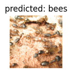
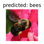
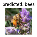
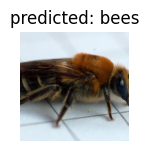
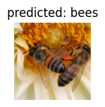
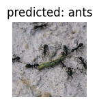
Let’s now visualize the inference of the trained model on some sample images from the validation step

def visualize_model(model, num_images=6):
    was_training = tf.keras.backend.learning_phase() == 1
    images_so_far = 0
    fig = plt.figure()

    for i, (inputs, labels) in enumerate(dataloaders['val']):
        inputs = tf.convert_to_tensor(inputs.detach().numpy())
        labels = tf.convert_to_tensor(labels.detach().numpy())

        outputs = model(inputs, training=False)
        preds = tf.argmax(outputs, 1)

        for j in range(inputs.shape[0]):
            images_so_far += 1
            ax = plt.subplot(num_images//2, 2, images_so_far)
            ax.axis('off')
            try:
                ax.set_title(f'predicted: {class_names[preds[j]]}')
            except:
                continue
            imshow(inputs[j])

            if images_so_far == num_images:
                model(inputs, training=was_training)
                return

    model(inputs, training=was_training)

visualize_model(transpiled_model)

Conclusion

We’ve just seen how the transpiler can be used to convert a model from PyTorch to TensorFlow and train the converted model in TensorFlow.

Head over to the Examples and Demos section in our documentation if you’d like to explore other demos like this. You can also run demos locally on your own machine by getting started or signing up for an API key to get a transpiler API key with juiced up usage quotas for local development.

If you have any questions or suggestions for other interesting demos you’d like to see, feel free to ask on our Discord community server, we look forward to seeing you there!